TL;DR
The best way to learn is to teach, so in this post I walk through an example of putting broadcasting to use in a heuristic number reading app. Part 1 of two in making my first neural network.
Overview
The code in this post is largely from the awesome lessons over at fast.ai, with the explanation all in my own words. Many thanks to that team for their amazing work. This is part one of two from the same lesson learning to make a digit classifier, the next will go into making the neural network that performs better at the same task.
What?
We’re going to make a function to act as a benchmark for a neural network. The task it will perform is to correctly identify a number, given a hand drawn picture of it.
Why?
You need to crawl before you can reject unripe tomatoes1, and that before you can comfortably learn to tie a necktie while your Tesla is whipping around corners with you in the drivers seat.
Who?
Who am I!? Who are you?!
How?
Using PyTorch2, an opensource toolkit for building neural networks. Truly the shoulders of giants at our finger tips.
Code Review
Making a neural network to solve a problem is a bunch of mumbo jumbo if we’re not actually performing better than a simpler heuristic function. To test that, we will start off by constructing a simple classification that classifies a digit based on which average digit image it is nearest to (You’ll see what I mean later). This will determine the score-to-beat with the neural network we make in the next post.
Let’s get into it!
The required dependencies!:scikit-learn, fastbook, matplotlib
Data Acquisition
In any real world ML application, data acquisition can be one of the more costly parts of the process, luckily not so for this simple learning example.
We’re using a variant of the classic NIST database, a collection of images of hand drawn numbers that provided the means for benchmarking in earlier days of ML.
I had trouble wrangling with the various sources for this database online, the simplest workable solution I could find for us to get a grip on these images was to just import the datasets library that comes with installing the scikit-learn package.
Pre-processing data before even touching any neural net methods can improve your final performance. Note the data set information offered at the source page:
We used preprocessing programs made available by NIST to extract normalized bitmaps of handwritten digits from a preprinted form. From a total of 43 people, 30 contributed to the training set and different 13 to the test set. 32x32 bitmaps are divided into nonoverlapping blocks of 4x4 and the number of on pixels are counted in each block. This generates an input matrix of 8x8 where each element is an integer in the range 0..16. This reduces dimensionality and gives invariance to small distortions.
Always good to get to know your data..
dict_keys(['data', 'target', 'frame', 'feature_names', 'target_names', 'images', 'DESCR'])What’s in here?
Code
(array([0, 1, 2, ..., 8, 9, 8]), '# targets: 1797')So we have 1797 numbers in this data set.
Code
([[0.0, 0.0, 5.0, 13.0, 9.0, 1.0, 0.0],
  [0.0, 0.0, 13.0, 15.0, 10.0, 15.0, 5.0],
  [0.0, 3.0, 15.0, 2.0, 0.0, 11.0, 8.0],
  [0.0, 4.0, 12.0, 0.0, 0.0, 8.0, 8.0],
  [0.0, 5.0, 8.0, 0.0, 0.0, 9.0, 8.0],
  [0.0, 4.0, 11.0, 0.0, 1.0, 12.0, 7.0],
  [0.0, 2.0, 14.0, 5.0, 10.0, 12.0, 0.0],
  [0.0, 0.0, 6.0, 13.0, 10.0, 0.0, 0.0]],
 array([[ 0.,  0.,  5., 13.,  9.,  1.,  0.,  0.],
        [ 0.,  0., 13., 15., 10., 15.,  5.,  0.],
        [ 0.,  3., 15.,  2.,  0., 11.,  8.,  0.],
        [ 0.,  4., 12.,  0.,  0.,  8.,  8.,  0.],
        [ 0.,  5.,  8.,  0.,  0.,  9.,  8.,  0.],
        [ 0.,  4., 11.,  0.,  1., 12.,  7.,  0.],
        [ 0.,  2., 14.,  5., 10., 12.,  0.,  0.],
        [ 0.,  0.,  6., 13., 10.,  0.,  0.,  0.]]))
And it looks like the ‘data’ entity is a list of one dimensional vectors, listing out the 64 pixels of each image, whereas the ‘images’ entity is the same info already organized into the 8x8 array of pixels.
The values in the arrays are from 0-16, as described in the source documentation. Important to keep in mind that we might want to normalize them all to a range from 0 to 1 for our purposes. We’ll do that later.
I had to do some funny indexing to tease that out. Something I learned along the way was the fantastic .view() function of the Tensor object in pyTorch. Tensors are like a numpy array, have a lot of features that will be critical for quickly creating neural nets. This object type was imported with fastbook.
tensor([[ 0.,  0.,  5., 13.,  9.,  1.,  0.,  0.],
        [ 0.,  0., 13., 15., 10., 15.,  5.,  0.],
        [ 0.,  3., 15.,  2.,  0., 11.,  8.,  0.],
        [ 0.,  4., 12.,  0.,  0.,  8.,  8.,  0.],
        [ 0.,  5.,  8.,  0.,  0.,  9.,  8.,  0.],
        [ 0.,  4., 11.,  0.,  1., 12.,  7.,  0.],
        [ 0.,  2., 14.,  5., 10., 12.,  0.,  0.],
[ 0., 0., 6., 13., 10., 0., 0., 0.]])Using -1 in the argument for the view function will auto-size the tensor based on the number of elements in the array, and the other dimensions specified. This should come in handy!
For a classification task such as this, it’s important to keep in mind that our data should be balanced in quantity per class. Let’s take a look at how many we’ve got.
Code
['0: 178',
 '1: 182',
 '2: 177',
 '3: 183',
 '4: 181',
 '5: 182',
 '6: 181',
 '7: 179',
 '8: 174',
 '9: 180']
So, a little imbalance but nothing crazy. Worth checking though…
If we train on a million images of 7’s, and only a thousand 1’s, we can be duped into thinking we’re rocking a 0.1% error rate by a naive model that guesses ‘7’ no matter what you give it!
Picturing Inputs


Turns out that pre-processing that comes baked in does make them pretty grainy. But nothing some training can’t solve.
Bucketing Classes
We need to separate out our inputs for training purposes. We’ll iterate across the ‘targets’ list, using the target numbers themselves as the index value to dump the corresponding ‘image’ data into the storage bin.
Code
stacked = []
# This loop because stacked=[[]]*10 makes 1 list in list, with 10 copies of pointers... need separate objects
for i in range(10):
    stacked.append([])
# Assign all images to the right collection in the 'stacked' list, indexed by target
for i in range(len(mnist["target"])):
    stacked[mnist["target"][i]].append(mnist["images"][i])
lens = [len(stacked[i]) for i in range(10)]
lens, min(lens)  # Confirm counts of samples
([178, 182, 177, 183, 181, 182, 181, 179, 174, 180], 174)So that worked, we now have a list of lists of arrays, the arrays being interpreted as images, the lists being collections of images, with all images in a given collection being an image of the same hand drawn number. And we see that we have the fewest samples of numbers 8’s, so we’ll take only that many samples (174) of every other image for our dataset.
Segmentation
The next step is to define which data will be our training, and our validation set. It was important to bucket out our data first so by randomly sampling our data we didn’t generate a validation set with a large imbalance in the number of classes to be tested in it.
First we convert to a tensor, then segment training from validation data. Arbitrarily taking 20 examples from each digit, so, 11.5% of the total data set towards validation.
We’ll print out the size of these collections and take a peek at a sample to make sure we indexed right.
Code
# To make dataset a tensor, make it same number of dimensions
stacked = tensor([x[:174] for x in stacked])
# Segmentation: Pull 20 of each digit out of training set
test = [dig[-20:] for dig in stacked]
train = [dig[:-20] for dig in stacked]
# Confirm counts of samples
[len(test[i]) for i in range(10)], [len(train[i]) for i in range(10)]
show_image(stacked[3][0])  # Check sample
<Axes: >
Nice.
It’s important to keep track of what’s what.
(list, torch.Tensor, torch.Tensor, [list, torch.Tensor, torch.Tensor])Ok so our top level containers for training/testing data are basic python lists. Within those, we have 10 collections, one for each integer. Those are Tensors. And then, each image (a collection of pixels unto itself) within those tensors, are also Tensor type objects.
Instead of a basic Python list, we will need the top level containers as tensors to leverage the pyTorch functionality built into them. luckily it’s an easy conversion
Code
(torch.Size([10, 154, 8, 8]), torch.Size([10, 20, 8, 8]))Now here is a crtiical piece, working with multidimensional arrays and keeping in mind what we understand these to be. Our test and training tensors have the same dimensionality but not the same size.
Building Benchmark Function
Where it gets fun now is in averaging and such across these dimensions. By doing so we can get the ‘average drawing of a number,’ which will be integral to creating our benchmark classification function.
The ‘Average’ Digit
Code


I hope you think this is as cool as I do! It calls to mind the idea of seeing a video of someone doing something routine every day like brushing their teeth, but at a million times speed, all the variations of movement wash out and create this somewhat blurry view of the general pattern. Like a mashing of all possible worlds. What did that code do, how did we get this? Let’s tear this one apart.
First of all, we’re dealing with a 4 dimensional tensor, train. When we jumped into a list comprehension iterating for x in train, we ‘stepped into’ that 0th dimension, so to speak. Then any given element x is a 3 dimensional tensor.
We will go through 10 of them, one for each integer, and each will contain 174 8x8 images. When we take the mean in the 0th dimension of x, we are saying “Across these 172 samples of 8x8 containers, what are the average values for element?” A visual way to think of this is that you have 174 pages, each with an 8x8 grid of numbers on it. We will reduce it to a single page by taking the average through all the pages, for each number; i.e. the 1st number on our single summary page will be the average of the 1st number from all of the 174 pages. The 2nd number will be the average of all the 2nd numbers, etc.
In practice, this means that the more samples in which a given pixel was inked, the darker that pixel will be in the average.
Least-Difference As Decision
Recall, our goal is first create a benchmark classification function that doesn’t use neural network methodologies. Now that we have the aberage, or ‘archetypal’ form of each digit, we can define a function to compare an input digit against the ideal digits to identify which it has the least difference with.
Since all of the ‘images’ we’re talking about are represented as a collection of 64 numbers, each number indicating a pixels brightness, taking the difference between two images as a whole just entails taking the difference between each pair of corresponding pixels from each, and then taking the average or using some other function to convert those 64 differences into one number.
Fortunately, the fastbook library again serves up a toolkit: the module F, containing functions we’ll need in our travels on any ML journey.
Let’s use the L1 loss and MSE as loss functions3. We’ll pass in the first example of a zero we have against the ‘average’ zero:

Code
('L1 loss: 1.9119317531585693', 'MSE Loss: 3.072631359100342')Other than validating the fact that we aren’t getting any errors due to bad inputs, this doesn’t tell us much. Generally, the MSE loss will always be greater than the L1 loss. Because loss increases exponentially with deviation from target, in principle, it is a better loss function as it will give a stronger learning signal in training; i.e. a step in the right direction will have greater effect on minimizing the loss function, at greater distance from target. But I’m getting ahead of myself here.
A more meaningful test that this is making sense would be to compare the error of a different sample digit against our ideal zero. Lets go with a seven.

Code
('L1 loss: 4.754464149475098', 'MSE Loss: 6.698919296264648')Seems about right- a random zero sample from the database has a lower measure of loss when tested against the average zero than a random seven does. Now that we know the measure is behaving, we’ll pack into a function so we can call on it and simplify our upcoming code. We’ll use the L1 norm:
I would really encourage you to simmer with the function defined in this code block and make sure you understand how it works: - We’re taking the difference of each element in each input by subtracting - We’re taking the absolute value of all those differences - We’re averaging across the last two dimensions of the tensor. Think about it… what happens if there is more than just two dimensions
Computing The Benchmark
Having the benchmark function, lets take it for a whirl. We will pass in the average digits as one tensor, and the training digits as the other. This is a critical point! A foundational strategy for the approach to neural nets is that we work with tensor-wise operations. Instead of taking the difference of one image against another, one at a time, we pass entire tensors into functions that compute across them. This becomes an absolute necessity for the sake of algorithmic and code execution efficiency.
RuntimeError: The size of tensor a (154) must match the size of tensor b (10) at non-singleton dimension 1An error! The error message points to a mismatch in the sizes of our tensors. Let’s take at these:
Right, our means contains 10 images, each 8 by 8 pixels, one image for each ‘average’ digit. Meanwhile train is storing our training data, so it has a collection of images for each digit. So the tensor has greate dimensionality because for each digit there are 154 images of 8x8 pixels.
The mnist_distance function we made subtracts every element in the input tensors, so it makes sense that there needs to be an equal number of individual elements for the computer to make sense of the instruction. When I say element in this context I mean the numeric value assigned to each pixel in each image indicating its brightness. So at first blush, we’d think we need to expand the means tensor so as to contain many copies of the each average digit.
How can we fix this? This reveals a critical lesson in the technique called broadcasting.
Broadcasting is a functionality pyTorch brings over from Numpy. From the docs:
The term broadcasting describes how NumPy treats arrays with different shapes during arithmetic operations. Subject to certain constraints, the smaller array is “broadcast” across the larger array so that they have compatible shapes. Broadcasting provides a means of vectorizing array operations so that looping occurs in C instead of Python. It does this without making needless copies of data and usually leads to efficient algorithm implementations.
Instead of using Python to make many copies of our average digits, we can just alter the structure of the tensor means in memory so as to make it compatible for computation with train. To do this, we use the unsqueeze function to add an extra dimension along which we will broadcast.
The way I look at this is like folders in a file system! In this diagram, the unsqueeze function added an extra layer to the nested boxes making up means.
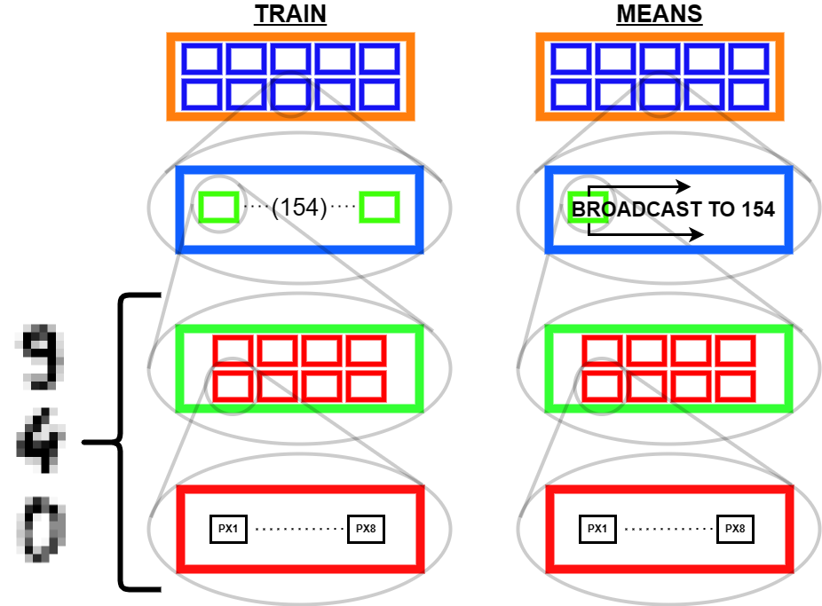
From the bottom up (i.e. right to left of tensor indices) we have:
- A folder with 8 numbers^(“files” in this analogy- the foundational stuff we are actually storing!) - the pixel brightness values for the 8 pixels in a single row.
- A folder with 8 of the preceding folders - one for each row of pixels making an image
- A folder with 154 of the preceding folders - In
train, the 154 different samples of hand written digits, for a given integer. Inmeans, a single box, redundant on its own, but serving as the thing to broadcast - A directory (our tensor) with 10 of the preceding folders, one for each integer
0through9
Lets test that this modified structure works:
Great, no error! We see the result is a tensor structured as an array of 10 vectors, each with 154 elements. In other words,a directory of 10 folders, each with 154 files.
We understand the numbers stored to be the L1 norm loss measures for each of the 154 samples of each digit, against the ‘average’ version of that digit. So by looking for the min and max values within these 10 vectors, we can identify the best and worst samples, as compared against their target digit:
Code


So we can get a sense for where this benchmark digit classification function might go wrong, such as by taking that worst 1 for a 7, or the worst 9 for a 4.
We’re close now. The goal here is a single performance measure, classification accuracy, for the benchmark function against all input data. That will be the score to beat with the neural entwork implementation.
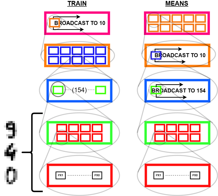
What we need to do is extend the logic of that last code segment, comparing each digit to not only the ‘average’ version of it’s target number, but also against the average version of every other number. To do this, we’ll have to broadcast some more. this is the structure we’ll use:
Code
Further unsqueezed shape of means: torch.Size([10, 1, 1, 8, 8])
Unsqueezed shape of train data   : torch.Size([1, 10, 154, 8, 8])
Why? Let’s go back to our norm function: def mnist_distance(a, b): return (a-b).abs().mean((-1, -2)) The last two dimensions will be averaged to get a score number, and we want a score number for every combination of sample image, and ‘average’ digits 0-9. Thinking of nested boxes again, we should expect the structure of our result tensor to have a path through it to each one of these combinations.4 To build this path, we first imagine it:
- The tensor as our outermost box should have 10 boxes in it, one for each ‘average’ digit; in this box that digit will be the comparison item against every sample.
- Within each of those boxes will be 10 more boxes, one for each of the sample pools (all samples of 0’s, all samples of 1’s, 2’s, etc.)
- Within each of those boxes will be 154 boxes, each containing the data for one sample image. The data is stored in array structure, i.e. 2 boxes, but we can leave it at that since at that level, all those 64 numbers per digit will be averaged out.
First of all, we unsqueeze the means tensor we had at the first index again so that the dimension where the differentiation between average digit occurs stays at the highest dimension. The result is that 10,1,1,8,8 tensor. We unsqueezed multiple times because we want copies of copies of each of the mean digits. One level of copying at the layer of sample pool, and copying againt to each sample image within the sample pool.
Next, we need to make the train tensor compatible with this. The thought is that this entire training set will be compared against each average, so there will need to be 10 copies of it. To achieve that we unsqueezed at the 0th index to allow for broadcasting to more copies.
The result is that the 10,1,1,8,8 tensor and 1,10,154,8,8 tensors are broadcast to be equal in shape to perform computation. First in dimension 1, the train data is broadcast (10 copies created), in dimension 2 the mean data is broadcast creating 10 copies of everything below. Then in the 3rd dimension, the means is again broadcast up to 154, creating 154 more copies of what is in the dimensions below. In this way, the 1st dimension corresponds to the different ‘ideal’ or mean digits 0-9, the 2nd dimension corresponds to all the data corresponding to the training data for digits 0-9. The 3rd dimension differentiates between individual samples of a given training digit. And the 4th and 5th dimension get us to individual pixels of those images.
Let’s see if it worked!
Code
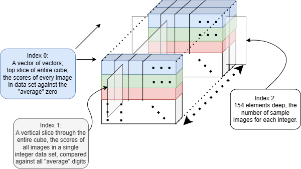
shape of all comparison: torch.Size([10, 10, 154])Great, no error!
The result is 3 dimensions instead of 5 because the mnist_distance function took the average across the last two dimensions, reducing the data in them to a scalar stored in the 3rd dimension. So for the 0th dimension, we have 10 collections of data (horizontal slices), which is the ideal digit is compared against the 154 samples for each digit as indexed in the 1st dimension (vertical slices), and the 2nd dimension (depth) indexing the 154 samples.
Picturing the 3D result as a cube, each element in the cube contains the numeric result from mnist_dist for the comparison of an ideal and a test image. Any given sample image is compared against all 9 ideal digits, and where the miniumum mnist_distance corresponds to the integer that the training digit actually is, the benchmark function was correct.
Alright, so we have a big tensor with every image compared against every ‘average’ digit. Now we need to do some smart indexing to identify the lowest loss function score for each sample image, indicating what number the benchmark function thinks that that image is, and to summarize all that output as a performance metric for us to beat.
Here are the lines in the following block where the maagic is baked into the cake: 3. Generalizing the function so it can handle inputs of varibable size 11. Using iterator to index an entire vertical slice of the data cube, yielding a 2D tensor. i) The .min(dim=0) looks across the 0th dimension of the input tensor, in this case the 2D array. It yields a tensor containing the minimum values in each slice. the .indices yields the indices at which those values were identified. ii) In the bigger picture, .min(dim=0) is looking at single columns of 10 numbers and returning the minimum value. 12. Tallying up how many classifications were attributed to each number 0 through 9. 13. Because our target values are number 0 to 9, they lend themselves to being used as indices. This same code for another kind of task might look very different. Here, our iterating/slicing strategy is such that we know the true digit for all the data points in iteration 0 are 0, iteration 1 are 1, etc, so we can simply take the number of classifications made to the current iteration number as the same thing as classifications to correct category, and add that to our running total.
Code
def acc_rslt(comp):
    c = comp.clone()
    x, y, z = [i for i in c.shape]
    totSamp = y*z
    totCorrect = 0  # Tallier
    confM = []  # confusion matrix will be result of stacking the bincount results
    for i in range(10):
        # Taking slice yields 2D object, shape (10,154), take min in each column (axis 1) to get digit prediction
        # Retrieve indices i.e. predictions for all comparisons
        # Yields a 1D tensor with count of integers indexed by integer
        id = c[:, i, :].min(dim=0).indices
        predCnt = torch.bincount(id, minlength=10)
        totCorrect = totCorrect+predCnt[i]
        confM.append(predCnt)
    confM = torch.stack(confM)
    return (totCorrect/totSamp*100), confM


acc, conf = acc_rslt(all_comparison)
print('accuracy: '+str(round(acc.item(), 2))+'%')

df = pd.DataFrame(conf)
df.style.set_properties(**{'font-size': '6pt'}).background_gradient('Greys')
df.style.set_table_styles([dict(selector='th', props=[(
    'text-align', 'center')])]).set_properties(**{'text-align': 'center'})
accuracy: 89.94%| 0 | 1 | 2 | 3 | 4 | 5 | 6 | 7 | 8 | 9 | |
|---|---|---|---|---|---|---|---|---|---|---|
| 0 | 153 | 0 | 0 | 0 | 1 | 0 | 0 | 0 | 0 | 0 |
| 1 | 0 | 124 | 8 | 1 | 0 | 2 | 4 | 0 | 4 | 11 |
| 2 | 0 | 6 | 136 | 4 | 0 | 0 | 0 | 2 | 5 | 1 |
| 3 | 1 | 0 | 1 | 143 | 0 | 0 | 0 | 4 | 2 | 3 |
| 4 | 1 | 3 | 0 | 0 | 143 | 0 | 0 | 7 | 0 | 0 |
| 5 | 1 | 0 | 0 | 1 | 1 | 131 | 3 | 0 | 0 | 17 |
| 6 | 1 | 1 | 0 | 0 | 1 | 0 | 151 | 0 | 0 | 0 |
| 7 | 0 | 0 | 0 | 0 | 1 | 1 | 0 | 152 | 0 | 0 |
| 8 | 0 | 15 | 2 | 2 | 0 | 4 | 2 | 2 | 119 | 8 |
| 9 | 0 | 3 | 0 | 5 | 4 | 1 | 0 | 6 | 2 | 133 |
Exciting! Just shy of 90% accuracy is the score to beat. And we can see which deigits performed better or worse. Row 8 shows that numbe r8 had the worst performance, with only 119/154 images classified correctly, with most 8’s being incorrectly classified as 1’s, or 9’s. Following that, 5’s had 131/154 correct, with 17 instances incorrectly classified as a 9. Now, we are ready to make a neural network.
If you want to understand each line of everything that follows, a strong grasp of broadcasting will be critical.
Outro
A couple of key take aways from this portion of the fastAI lesson. A notable one not to skip si the fact that there is no sense deploying neural networks if other methods can do the job better, so we should always be verifying that we perform better than the alternatives. I really had a few a-ha moments in learning about the broadcasting techniques and so I felt it would be great to share. It was a lot easier to scribble the drawings on paper than to put them on the screen but I hope you find them illuminating!
I was able to create that neural net to classify digits more accurately, in the end. I’ll walk through that in the next post.
Footnotes
Too fun not to share though I think this is a machine vision implementation without neural nets. Probably just averaging colour across a pixel range to trigger the paddles.↩︎
If it ain’t ‘py’, it ain’t python, right?↩︎
Check out this link for more on these norms. Be aware that MSE is just a colloquial name for the L2 norm, and also that a norm alone isn’t a ‘loss function’ per se. Any function at all is a loss function if you use it to calculate loss. That cetainly doesn’t mean it’ll be a good one. Books could be written on the topic though, so we’ll leave it there.↩︎
There is some ambiguity as to how we could’ve gone about this, as to wehther or not we thought about the digit from which samples are drawn as the first layer, or the average digit being tested against as the first layer. I chose the latter.↩︎